Rounding errors in softmax and cross-entropy
A classifier produces scores for possible answers. Softmax converts those scores into probabilities. Cross-entropy compares the probabilities with a target and supplies a loss for training. PyTorch accepts either a correct class or a target probability distribution in its cross-entropy function.
The arithmetic has finite precision. A calculation can discard a small difference even when that difference can be stored on its own. Changing the order of operations can change the result. PyTorch describes this constraint in its numerical accuracy notes.
In A Fix for Softmax and Cross-Entropy, Jonathan T. Barron, Dan Gnanapragasam, and Michael Tschannen examine two consequences for training. They call them Softmax Collapse and Softmax Cancellation. Their examples and reformulations are the starting point for this post. We will work through a product-classification example and translate the supplied JAX code into PyTorch.
The numerical-error measurements use PyTorch 2.14.1 with float32 tensors on an ARM64 CPU. Reference calculations use 80 decimal digits of precision. The saved results record the inputs, outputs, and implementation checksum. Different hardware or implementations can produce different residuals. The introductory classifier uses float64 to illustrate the calculation before we examine float32 rounding.
A neural network classifier
A neural network, or NN, combines input values through layers of trainable weights. A weight multiplies an incoming value. A bias adds an offset. A hidden layer computes intermediate values before the output layer produces a score for each class. PyTorch’s network tutorial follows this structure.
Imagine classifying a package as product A or product B. For this arithmetic example, choose two input feature values $x=[1,0.5]$. These are illustrative measurements. We also choose the weights by hand, so this example makes no claim about recognition accuracy on real images.
The hidden units compute $h_1=\operatorname{ReLU}(x_1)$ and $h_2=\operatorname{ReLU}(2x_2)$. ReLU keeps positive values and replaces negative values with zero. Both hidden outputs are one. The output weights give $z_A=h_1+h_2=2$ and $z_B=0$. All biases start at zero. The classifier record contains every chosen parameter.
0.8808Product B 0.1192−log(0.8808) ≈ 0.1269Score gradients [−0.1192, +0.1192]
Product A has the higher score. Softmax assigns it probability $0.8808$, and the loss for a correct A label is approximately $0.1269$. The network predicts the right product but can still increase its probability. The next section derives the gradients that ask it to do so.
The diagram shows probabilities to explain the calculation. In PyTorch, pass the raw scores to F.cross_entropy, which combines normalization and the loss computation. The classifier script builds this network and records the bias updates below.
From scores to a training gradient
Suppose a model must identify a grocery product from an image. A logit is the model’s score for a candidate product before normalization. Write the scores as $z_i$, where $i$ identifies a product. Softmax gives each product a probability $q_i$.
\[q_i = \frac{e^{z_i}}{\sum_j e^{z_j}}.\]The denominator adds the exponentials for all candidates. Dividing by this sum makes the probabilities add to one. Increasing a score relative to the others increases its probability.
Let $p_i$ be the target probability for product $i$. A hard target places all target probability on the correct product. A soft target can distribute it across several products. Cross-entropy is
\[L = -\sum_i p_i\log q_i.\]We use the natural logarithm throughout. For a hard target, the loss reduces to $-\log q_t$, where $t$ is the correct product. Increasing that product’s probability reduces the loss. These definitions follow the PyTorch cross-entropy specification.
The gradient with respect to a score measures how the loss changes when that score changes. We can derive it by writing the loss in terms of the scores. Since the target probabilities sum to one,
\[L = \log\left(\sum_j e^{z_j}\right) - \sum_i p_i z_i.\]Differentiating with the target held fixed gives
\[g_i = \frac{\partial L}{\partial z_i} = \frac{e^{z_i}}{\sum_j e^{z_j}} - p_i = q_i-p_i.\]Gradient descent subtracts the gradient. A negative entry asks for a higher score. A positive entry asks for a lower score. These instructions add to zero in exact arithmetic
\[\sum_i g_i = \sum_i q_i-\sum_i p_i = 0.\]This also follows from the scores themselves. Adding the same constant to every score leaves all their differences unchanged. It leaves the probabilities and loss unchanged too.
A slice of the loss landscape
A loss landscape maps parameter settings to loss values. To draw one for our classifier, hold the input and all connection weights fixed. Change only the output biases $b_A$ and $b_B$. The product scores become $[2+b_A,b_B]$. For the correct A label, the loss is
\[L(b_A,b_B)=\log\left(1+e^{b_B-(2+b_A)}\right).\]The horizontal axes below are bias settings. Height is the loss on this one example. The contour plot shows the same values from above. Each contour connects settings with equal loss.
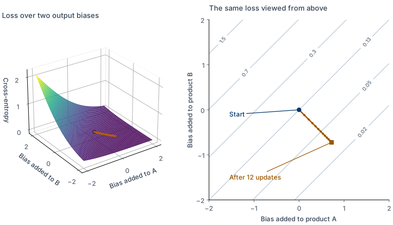
We can calculate the first update by hand. At the initial setting,
\[q_A=\frac{e^2}{e^2+1}\approx0.8808, \qquad q_B=\frac{1}{e^2+1}\approx0.1192.\]Each output bias contributes directly to its product’s score, so its gradient is the corresponding score gradient. Subtract the gradient with a learning rate of one
\[\begin{aligned} b_A' &= 0-(0.8808-1)\approx+0.1192,\\ b_B' &= 0-(0.1192-0)\approx-0.1192. \end{aligned}\]The recorded loss falls from $0.1269$ to $0.1013$ after this update. Increasing A’s bias and decreasing B’s bias widens the score gap in favor of the correct answer. After the recorded sequence of twelve updates, the loss is $0.0314$.
This slice has no finite point where the loss reaches zero. As A’s advantage grows, the loss and its slope become smaller. The smooth slope is useful context for the next example, where rounding makes one gradient component disappear.
A confident prediction by hand
Consider products A and B. Product A is correct. Give them scores
\[z=[20,0], \qquad p=[1,0].\]First subtract the largest score from both entries. This leaves the probabilities unchanged because the common exponential factor cancels between numerator and denominator. The shifted scores are $[0,-20]$. This shift avoids exponentiating the large positive score.
Write $a=e^{-20}$. The reference calculation gives
\[a \approx 2.061153622\times10^{-9}.\]The probabilities and gradients are
\[\begin{aligned} q_A &= \frac{1}{1+a}, & g_A &= \frac{1}{1+a}-1,\\ q_B &= \frac{a}{1+a}, & g_B &= \frac{a}{1+a}. \end{aligned}\]To the digits shown, the gradient is
\[g\approx[-2.061\times10^{-9},\;+2.061\times10^{-9}].\]Both entries are small because the prediction already favors the correct product. There is still an instruction to increase A’s score and decrease B’s score.
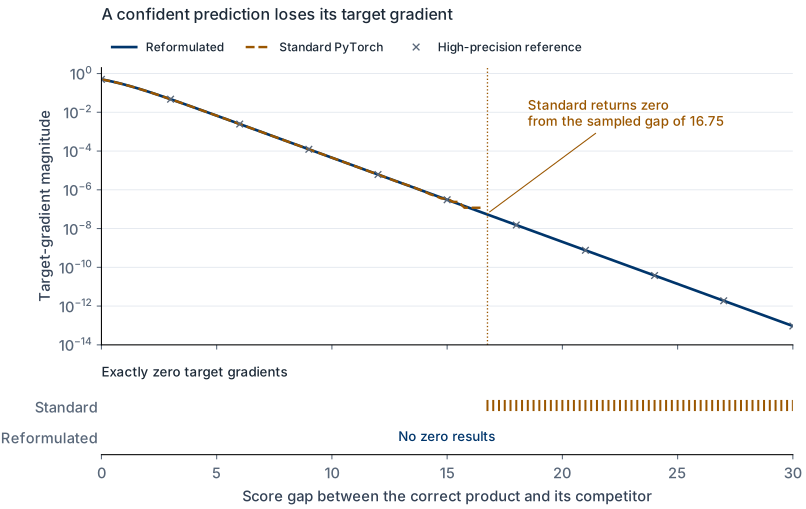
Now carry out the same steps in float32. The spacing from one to the next larger representable number is about $1.192\times10^{-7}$. Our value of $a$ is less than half that spacing. Adding it to one rounds back to one. The recorded arithmetic gives
\[1+a\;\longrightarrow\;1, \qquad q_A\;\longrightarrow\;1, \qquad g_A\;\longrightarrow\;0.\]The numerator for B still contains $a$. Its gradient survives. The computed loss also becomes zero because $-\log 1=0$.
This is Softmax Collapse. The loss still asks for a lower B score but loses the corresponding instruction to raise A’s score. The gradient entries no longer add to zero.
| Quantity | Standard | Reformulated |
|---|---|---|
| Loss | 0 | 2.061e−9 |
| Correct product gradient | 0 | −2.061e−9 |
| Competitor gradient | 2.061e−9 | 2.061e−9 |
The standard target gradient is zero. Its competitor gradient remains positive.
Keeping the small term
Rearrange A’s gradient before evaluating it
\[\frac{1}{1+a}-1 = -\frac{a}{1+a}.\]The right-hand expression retains $a$ in its numerator. Even if its denominator rounds to one, the result remains approximately $-a$. We can represent that number in float32.
The loss needs the same care. Calculating log(1 + a) first forms the rounded sum. log1p(a) evaluates $\log(1+a)$ with better accuracy for small inputs. In this example it preserves the loss of approximately $2.061\times10^{-9}$.
This rounding mechanism was documented in PyTorch issue 113708 in November 2023. Jason Gross proposed removing the maximum term from the exponential sum and using log1p for the remaining contribution. The underlying log-softmax issue therefore predates the newer paper. That issue concerns the first failure discussed here.
How slingshot updates arise
The slingshots mentioned in Barron’s thread concern training over time. A loss trace plots the losses encountered as the weights change. Thilak and colleagues documented recurring periods of low loss followed by weight growth and loss spikes. They also studied grokking, where performance on unseen examples improves long after training examples have been learned. A loss spike alone does not establish that improvement.
An optimizer converts parameter gradients into weight updates. Adam keeps running averages of the gradient and its square. For one weight, the gradient-based part of the update has the form
\[\Delta w=-\eta\frac{\widehat m}{\sqrt{\widehat v}+\epsilon}.\]Here $\eta$ is the learning rate. $\widehat m$ averages the weight’s gradients and $\widehat v$ averages their squares, with corrections for starting the averages at zero. The positive constant $\epsilon$ limits division by a small denominator. Weight decay is an additional update that shrinks weights. These operations are specified in AdamW.
Barron and colleagues give this explanation for their experiments. When high-confidence gradients disappear, the stored squared-gradient average can decay. Weight decay or residual updates can move scores back across the rounding boundary. Returning gradients then meet a small denominator. The resulting update can raise the loss and restart the cycle. Their reformulation removes the abrupt loss of the target gradient. The behavior depends on the optimizer and its state.
- Target gradient rounds to zero
- Adam's gradient scale shrinks
- Target gradient returns
- Normalized update grows

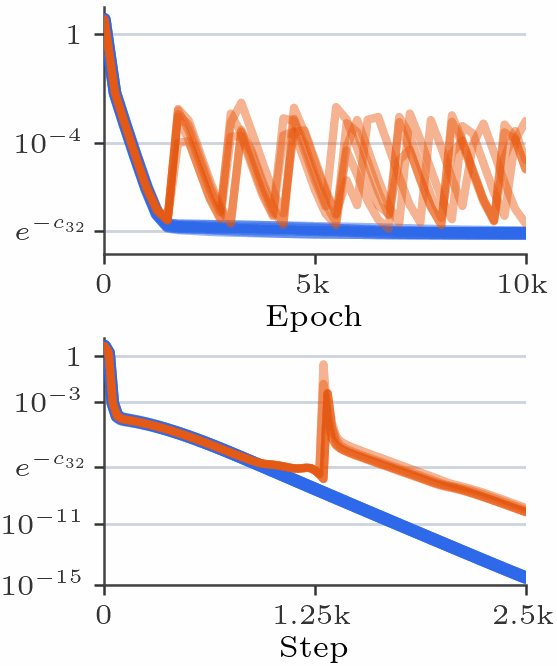
In the published plots, CE means cross-entropy. Epoch counts passes through the training data. Step counts optimizer updates. The symbol $c_{32}$ is the paper’s float32 score-margin threshold. The marked level $e^{-c_{32}}$ indicates its corresponding small-loss scale. The toy classifier’s bias updates above have no slingshot. The published traces show experiments in which the loss calculation interacts with adaptive optimization over training.
Hard targets in PyTorch
For more than two products, collect the competing scores relative to the target
\[r = \log\left(\sum_{j\ne t} e^{z_j-z_t}\right).\]Then the loss is
\[L=\log(1+e^r)=\operatorname{softplus}(r).\]Log-sum-exp means the logarithm of a sum of exponentials. Softplus is the function $\log(1+e^r)$. PyTorch provides implementations that avoid forming large exponentials directly. See logsumexp and softplus.
The function below takes logits with classes on the last axis. The integer target identifies the correct class for each example. It returns a loss per example, so call .mean() to average a batch. The examples assume finite float32 or float64 logits and at least two classes.
1
2
3
4
5
6
7
8
9
10
import torch
import torch.nn.functional as F


def hard_cross_entropy(z, target):
    index = target.unsqueeze(-1)
    target_score = z.gather(-1, index)
    mask = torch.zeros_like(z, dtype=torch.bool).scatter(-1, index, True)
    others = (z - target_score).masked_fill(mask, -torch.inf)
    return F.softplus(torch.logsumexp(others, dim=-1))
The mask removes the target from the exponential sum because $e^{-\infty}=0$. The target score now enters the calculation through its differences from the competing scores. Automatic differentiation collects its gradient as the negative sum of the competitors’ contributions.
Run the worked example
1
2
3
4
5
6
7
z = torch.tensor([20.0, 0.0], dtype=torch.float32, requires_grad=True)
target = torch.tensor(0)

loss = hard_cross_entropy(z, target)
gradient, = torch.autograd.grad(loss, z)
print(loss.item())
print(gradient)
The saved run gives a loss of approximately 2.061e-9 and gradients [-2.061e-9, 2.061e-9]. F.cross_entropy gives zero loss and gradients [0, 2.061e-9] for the same inputs.
The winning probability may still round to one if we store it as a float32 number. Its small log-probability and gradient remain representable. Preserving those quantities is what changes this training calculation.
When a student matches its teacher
In knowledge distillation, a student model is trained to match a teacher’s outputs. The target can express uncertainty across several products. This use of soft targets is described by Hinton, Vinyals, and Dean.
Keep the teacher fixed. Let $p$ be its probabilities and $q$ the student’s probabilities. The gradient with respect to the student scores remains $q-p$.
Take identical teacher and student logits
\[z_T=z_S=[0,1,2].\]Subtracting the largest score gives $[-2,-1,0]$ for both. Their probabilities therefore have the same expression
\[p=q=\frac{[e^{-2},e^{-1},1]}{e^{-2}+e^{-1}+1}.\]By hand, each gradient is a number minus itself. Every entry should be zero. The cross-entropy loss remains the teacher’s entropy, $-\sum_i p_i\log p_i$, which measures the uncertainty of its distribution. Matching the teacher minimizes this loss without requiring the loss to be zero.
We can check the matching case in PyTorch
1
2
3
4
5
teacher = torch.tensor([0.0, 1.0, 2.0], dtype=torch.float32)
student = teacher.clone().requires_grad_()
loss = F.cross_entropy(student, teacher.softmax(dim=-1))
gradient, = torch.autograd.grad(loss, student)
print(gradient)
The saved run returns approximately
\[g=[7.451\times10^{-9},\;1.490\times10^{-8},\;5.960\times10^{-8}].\]The teacher’s forward probabilities and the student’s backward calculation can follow different sequences of rounded operations. For example, dividing exponentials by their sum and exponentiating a log-softmax need not give identical stored values. When those values differ, their subtraction leaves a residual. Subtracting identical stored arrays would give zero.
If the logits are close rather than identical, rounding errors can obscure part of the desired difference. The figure compares both cases using the recorded PyTorch outputs.
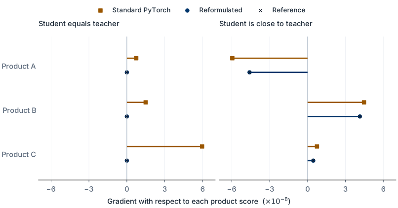
The left panel establishes a residual update where the matching objective calls for none. The right panel shows that the discrepancy also affects the size of an update before the student reaches the teacher. Neither panel measures an effect on model accuracy. These are checks of the loss and its derivative.
Compute the difference before converting to probabilities
Start with the difference between student and teacher logits
\[\delta_i=z_{S,i}-z_{T,i}.\]For identical finite inputs, $\delta_i$ is exactly zero. To connect this difference with the probabilities, substitute $z_S=z_T+\delta$ into softmax
\[q_i=\frac{p_i e^{\delta_i}}{\sum_j p_j e^{\delta_j}}.\]Let $s_i=\log(q_i/p_i)$ be the log probability ratio. We can recover the required gradient through
\[q_i-p_i=p_i(e^{s_i}-1).\]expm1(s) calculates $e^s-1$ with accuracy near zero. It avoids forming an exponential that rounds to one before subtracting one.
For the implementation, subtract the teacher-weighted average of the logit differences. This gives $d_i=\delta_i-\sum_j p_j\delta_j$. Subtracting a shared value cancels in the probability ratio above. Since $\sum_j p_j=1$, we can write
\[s_i=d_i-\operatorname{log1p}\left(\sum_j p_j\operatorname{expm1}(d_j)\right).\]At identical logits, $d_i=0$, $s_i=0$, and $p_i\operatorname{expm1}(s_i)=0$. The result follows through the calculation without subtracting independently rounded probability estimates.
Soft targets in PyTorch
We first need the reformulated log-softmax. Its structure matches the hard-target calculation, with the largest score selected as the reference.
1
2
3
4
5
6
7
8
def stable_log_softmax(z):
    index = z.argmax(dim=-1, keepdim=True)
    maximum = z.gather(-1, index)
    mask = torch.zeros_like(z, dtype=torch.bool).scatter(-1, index, True)
    shifted = torch.where(mask, 0.0, z - maximum)
    others = shifted.masked_fill(mask, -torch.inf)
    log_other_mass = torch.logsumexp(others, dim=-1, keepdim=True)
    return shifted - F.softplus(log_other_mass)
The next function computes the probability difference through the logit differences when the distributions are close. It uses direct subtraction for entries with larger log probability ratios. The correction in g reduces any residual in the sum of the gradient entries. Floating-point rounding still applies to that correction.
1
2
3
4
5
6
7
8
9
10
11
12
13
14
15
16
17
def soft_cross_entropy(student, teacher):
    with torch.no_grad():
        log_q = stable_log_softmax(student)
        q = log_q.exp()
        p = stable_log_softmax(teacher).exp()
        delta = student - teacher
        d = delta - (p * delta).sum(dim=-1, keepdim=True)
        s = d - torch.log1p(
            (p * torch.expm1(d)).sum(dim=-1, keepdim=True)
        )
        near = s.abs() < 1
        small_s = torch.where(near, s, 0.0)
        u = torch.where(near, p * torch.expm1(small_s), q - p)
        g = u - q * u.sum(dim=-1, keepdim=True)
        loss = -(p * log_q).sum(dim=-1)

    return loss + (g * (student - student.detach())).sum(dim=-1)
torch.no_grad() keeps the teacher fixed and prevents differentiation through the gradient calculation. The final line supplies the calculated student gradient. student - student.detach() has a forward value of zero. Its derivative with respect to student is one because detach() removes the second term from the differentiation graph. Multiplying by g therefore preserves the forward loss and supplies g during the backward pass.
Run the matching-teacher example with the new function
1
2
3
4
student = teacher.clone().requires_grad_()
loss = soft_cross_entropy(student, teacher).mean()
gradient, = torch.autograd.grad(loss, student)
print(gradient)
It returns [0, 0, 0] in the saved run. The loss remains approximately 0.8324, consistent with the entropy of this teacher distribution.
The complete Python file contains the functions and runnable examples. They use classes on the last axis and return one loss per example. The soft-target function supplies first-order student gradients and freezes the teacher. Its detached gradient construction does not support second derivatives. Class weights, ignored labels, label smoothing, and mixed-precision execution require separate handling.
Conclusion
In the confident prediction example, adding the competing probability mass to one discards a term that the target gradient still needs. In the teacher example, rounded probability calculations leave a residual at a point where the matching objective has zero gradient. The reformulations preserve the relevant differences in the measured examples.
Our checks compare loss values and gradients with a higher-precision reference. They also cover tied scores, incorrect predictions, batched averaging, and a fixed teacher. They do not establish a training-speed or accuracy improvement for a particular model. The source paper reports training experiments separately.
Before using a reformulated loss in training, check its values and gradients against a higher-precision reference on confident predictions and matching teacher outputs in your own execution environment.